HYDROLOGIC MODELING
Methodology
The specific objectives of this section are:
- Develop a conceptual model of the study site.
- Use available sensor observations to calibrate the related numerical model to mainly estimate hydraulic properties of the area.
- Apply the model for the following:
a. Evaluating the causes for the slow drainage and suggesting mitigation actions.
b. Assessing drainage in the case of a surface runoff flooding scenario
c. Examining the effect of sea level rise
d. Estimating flow budget under different scenarios
The Conceptual Model
The approach utilized available and newly collected data in developing the site model. Limited available data included geographic information data (aquifer and watershed delineations, land cover/use, surficial geology, and soil)[21] and a 10 meter resolution digital-elevation model (DEM)[22]. A number of wells exist but they are located outside the study area so they were just used to infer water level near the Pond. Figure 17 displays the area, which is extended far from the Pond due to the absence of nearby natural inland boundaries.
As is the case for any hydrological system, surface and subsurface inflows and outflows occur at the boundaries of a pond or at the ground surface due to rainfall recharge and surface water flow. These direct water inflows and outflows are schematically illustrated in Figure 27. Most of these are not directly measured, such as surface runoff and groundwater discharge. An alternative for groundwater discharge in Figure 28 is to set aquifer water level at the area’s boundary inferred from the available data and adjusted based on model calibration. A baseline value of 9 m was assigned at such a boundary. Known tide measurements were assigned to the ocean boundary. Ocean discharge is estimated by the model based on the tide levels and aquifer water levels as well as hydraulic conductance of the material at the ocean land interface. Hydraulic conductance is related to hydraulic conductivity of the boundary material. Flow across the boundary is proportional to the water level difference across the boundary, and conductance is the constant of the proportionality.
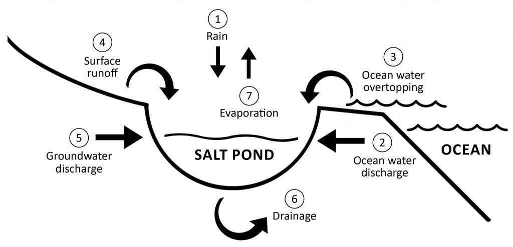
(Figure 27. A schematic plot illustrates various inflows, which can cause flooding. The flow occurs due to the interaction between the Pond and both the ocean and the groundwater aquifer (An aquifer is defined as a geological subsurface formation that allows water flow and storage). Note that ocean water discharge can be reversed as outflow, which is the main Pond drainage mechanism. It occurs when the water level in the Pond is higher than the ocean level. On the average, water flows from land towards the ocean, with varying flows at the ocean depending on tide fluctuations and water-levels in the Pond. Also not shown are Pond evaporation and vertical loss through the Pond bottom. The latter is expected to be small due to the low conductivity of the clay material. The conceptual model requires setting a bottom for the modeled area where a no flow condition exists, which is not physically known in our case. A common practice is to set that deep enough so it would not interfere with the flow in the area.)
The Numerical Model
The study utilized the flow software (aka numerical model) MODFLOW (Harbaugh et al. 2000)[23]. The numerical modeling adopted requires dividing the modeling area into a three-dimensional grid, which is shown in Figure 28a. The area’s top elevation follows existing topography while its bottom has a flat elevation of 500 m below msl. The active aquifer interacting with the Pond is limited to a much shallower depth, but it is unknown. Thus, and as was the case with the spatial extent, we chose to go much deeper to make sure the water at the ocean-land interface is free to move in such an area including interacting with the Pond (Figure 27). An optimal, variable-size grid was utilized, which was refined around the Pond area in order to attain higher accuracy (Figure 28b). The x-y plane sizes ranged between 15 and 100 m, while the vertical (z) sizes ranged between one meter at the top and 50 m at the bottom, with a gradual increase downward. The one-meter resolution for the top three layers was adopted to allow for accurate representation of the geophysical investigation. The software package interface GMS (https://www.aquaveo.com/software/gms-models-utilities) was used in facilitating the modeling process.
*Data input to the model included aquifer information, which in general are spatially distributed, such as hydraulic conductivity and specific yield. These will be estimated through the calibration process.
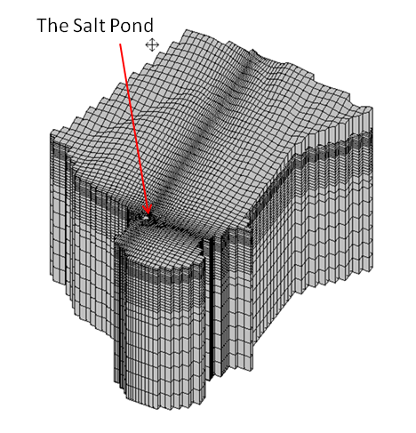
(Figure 28a. The numerical model three-dimensional grid.)
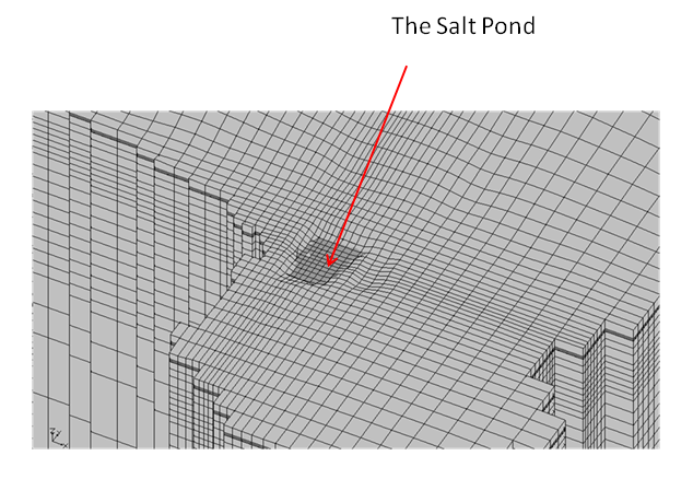
(Figure 28b. A zoomed-in view around the Pond area illustrating the refined three-dimensional grid. *Data input to the model included aquifer information, which in general are spatially distributed, such as hydraulic conductivity and specific yield. These will be estimated through the calibration process.)
Model Calibration and the Baseline Condition
The objective of calibration is to estimate model parameters, mainly those that cannot be directly measured. The calibrated model was used to meet the study objectives outlined above.
Calibration data included water-level sensor observations, which were collected during 2021 and 2022. In model calibration, we utilized the data collected between January and September 2022, which included an inundation anomaly in January 2022, which was likely due to a precipitation/surface water runoff event. According to the Hawaiʻi Climate Data Portal, the Eleʻele rain station, there was a significant rain event during January 1 – 4, peaking on January 3rd, with an approximate rainfall total of 13 centimeters[24]. Despite some inaccuracies in the water level sensor in the form of data scattering, the trend indicates a near sudden rise in water level in January. That rise, about 0.17 to 0.3 m, was followed by gradual decreases over about 30-60 days for the nodes shown in Figure 29. Fluctuations due to tides (of 1.0 m range) are in the order of two centimeters, indicating a relatively small ocean exchange, as also supported by the geophysical investigation.
A calibration effort was completed to estimate the hydraulic conductivity and specific yield for the aquifer. Based on the results of the geophysical study Figure 30), the aquifer was vertically divided into a total of four formations. The top three were treated as clays of one-meter thickness each, with lower hydraulic conductivity values, while the fourth was assumed as basalt of much higher conductivity. Hydraulic conductivities of the top three layers were assumed to be inversely proportional to the resistivities displayed in Figure 30.
Two cases were tested at the ocean boundary, namely a specified head or a head-dependent condition. The latter option requires assigning a hydraulic-conductance value reflecting the case where flow into and out of the modeled area is controlled by the ocean-side material, which has likely been reduced by illegal vehicular traffic over the years. The head-dependent boundary option was more realistic and the calibrated values were used in simulating the inundation anomaly case and for assessing various scenarios.
Results
Calibration
The calibration process includes a trial and error approach to estimate a set of parameters that provide the best match between measured and estimated variables, which are the sensor-measured water levels in this case. The values tried are constrained within literature values. The calibrated conductivities that gave the best match were 10-4, 5·10-5, 7.5·10-5, and 100 m/day, for the top three layers and the bottom formation, respectively. The values for clay agree with those listed by Fetter (2018)[25], which fall in the range of about 10-6 to 10-3 m/day. The head-dependent boundary best represents the measured small fluctuations in water levels, which are in the order of a few centimeters. A hydraulic conductance of 5 m/day gave the best results, which is a small value in comparison to a specified head case that implies an infinite conductance.
Figure 31 illustrates the relationship between ocean-boundary hydraulic conductance and estimated water levels at node 103 for the baseline case, under a steady state condition. Obviously a higher conductance will be beneficial in mitigating slow drainage. Unfortunately, the location of the baseline water level was not known, which would have helped in estimating the value of the conductance by plugging the value in the figure. A depth value of 0.73 m above msl was estimated based on the value of conductance of 5 m/day, which provided the best calibrated results. In the limit, as the conductance is large, the expected water level should be around 0.25 m above msl.
Due to the relatively small aquifer fluctuations in response to tides, and for simplification purposes, tides were overlooked in the following analyses. As can be seen in Figure 32, the match is reasonable regarding the observed initial rise in water level of about 0.2 m, and the time of decline occurring within 2 months. However, the model was not able to match the near linear decline shown in this figure and at all nodes (Figure 29). According to model theory and assumptions, the rate of change of water level should not be constant, but should be declining with time as the water level decreases. So it seems the flow to the Pond is complex and cannot be precisely simulated. However, the results in Figure 32 are reasonable towards serving the overall objectives of the project.
Model Applications
Assessing drainage in the case of a surface runoff flooding scenario
Figure 33 illustrates the time decline in the Pond following a sudden rise of 0.25 and 0.5 m above the baseline level, following a heavy storm. The rise is assumed to occur due to the combined effect of surface runoff and direct rain over the Pond. The water level needed about four months to recede back to the baseline level.
Effect of an increase in groundwater discharge
We also simulated a case of an increase in discharge due to wet conditions in the mountain side resulting in an increase of the water level by one meter. A modest increase of about 0.1 m occurred at the Pond site.
Effect of sea level rise
We simulated a sea level rise of 0.6 and one meter, which resulted in an increase in the water level at the Pond by about 0.8 and 0.5 m above the baseline level, respectively. Figure 34 illustrates the water levels in the area for the two cases. The figure also shows a flooded Pond under these circumstances.
Flow budget under different scenarios
For a transient (or time dependent) condition, water level would obviously rise when the input flow is larger than the output flow, and vice versa. The net change in storage is illustrated in Figure 35 for the case simulated in Figure 32. The results are consistent with the initial larger increase in water level due to a net positive change in storage. However, gradual decrease in the level will follow as the net change in storage is declining. The net change approaches zero (inflows equal outflows) after about 30 days at which the water level returns to the baseline value. It should be noted that tides are overlooked in this case. With tides, the flow would change directions at the shoreline depending on the relative magnitudes of water level in the aquifer and ocean level. In this case fluctuations would occur but the trend should be similar to that in Figure 35.
The transient simulations are required for cases that include limited time occurrence, such as overtopping or surface flows due to rain storms. On the other hand, a steady state or equilibrium condition represents invariant hydrologic conditions, such constant discharge or recharge. In this case, water inflows would equal outflows. However, the water level at the Pond would change from the baseline value by an amount that depends on the scenario under consideration. Table 1 provides the relevant data for some of the scenarios simulated here. Sea level rise provides the most significant increase in the Pond water level with a value of 0.8 and 0.73 m relative to the baseline case for sea level increase of one meter and 0.6 meter, respectively.
Discussion
Model limitations
- We considered developing a higher resolution survey of the Pond and surrounding area for topography. However, the scale of the model, which covers a much larger area than that of the Pond, made such details unnecessary.
- Flow density dependence was overlooked considering the small exchange was ocean water and the drastic difference between ocean and Pond salinities.
- The data regarding transient mauka water fluxes and or levels inferred from geophysical surveys were not available and relevant conditions we calibrated instead.
- The spatial extent of the clay layers is not known and hopefully more information will be added later in the model.
- As with any model, calibration results are not unique, and different combinations of parameter values can produce the same accuracy. For example, under idealized conditions, aquifer tide response depends on the ratio between conductivity and specific yield and not individually on each[25].
Modeling Conclusion
The modeling results show that the effects of direct surface flows on flooding exceed those due to subsurface flows. Surface flows are caused by direct rain, storm surface runoff, and ocean overtopping. Thus, mitigation should be mainly aimed at reducing surface runoff and ocean overtopping. The former could possibly be achieved by constructing a concrete trench upstream of the Pond, or other engineered solutions but these can be expensive and require time consuming government approval. To mitigate ocean overtopping, raising the beach berm is required. Slow drainage is likely due to the beach compaction occurring over the years or the possibility of an intrusion of the clay existing in the Pond. A high resolution geophysical investigation along the beach would be needed to validate such a condition. If needed, an approach to increasing the hydraulic conductance targeting the top few meters should be discussed with a geotechnical engineer.
Conditions under sea level rise are challenging to mitigate because the flooding is likely to cover the whole peninsula. In addition, as inferred from steady state simulations, Pond drainage would be only limited to low tides, which is not significant due to the relatively insignificant exchange between the Pond and the ocean.
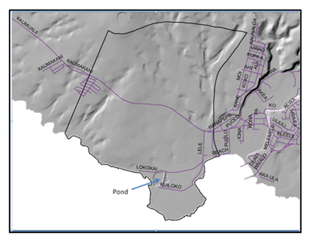
(Figure 26. Digital Elevation Model of the area and the modeling domain (black line).)
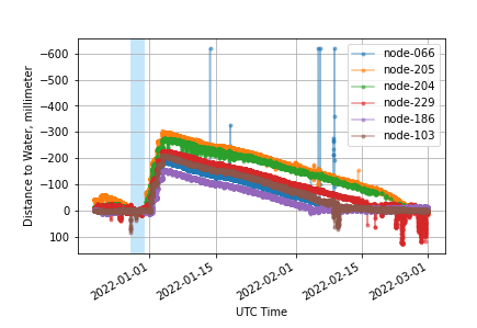
(Figure 29. Detail of inundation anomaly from January 2022, simultaneously depicting six of the working water level sensors (node-235 had previously failed). Shaded region identifies time period selected to artificially zero all gauges relative to each other. Deviations in peak water level height, or time until peak and time for water retreat are explained by spatial differences in how the area floods and how waters recede. Node-205 measured the largest change in water level, while node-186 measured the least.)

(Figure 30. Geophysical results along line BS that provides more detailed information on small-scale structures of the clay layers in the top ~4 m of the Pond.)
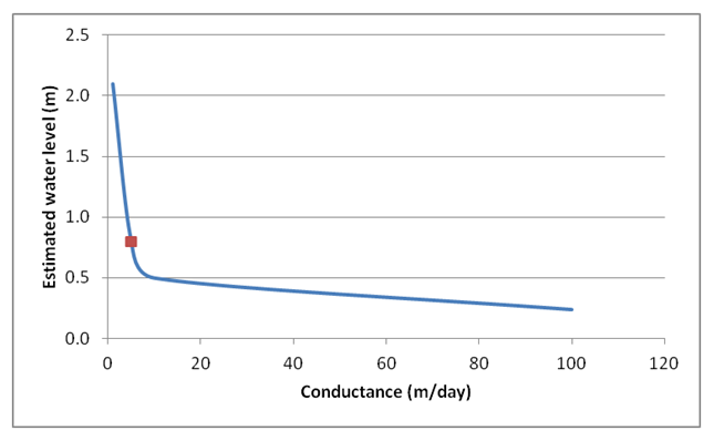
(Figure 31. Estimated water level at node 103 as a function of the conductance of the ocean boundary. The marked point illustrates the calibrated conductance value (5 m/day) and the corresponding water level (0.73 m).)
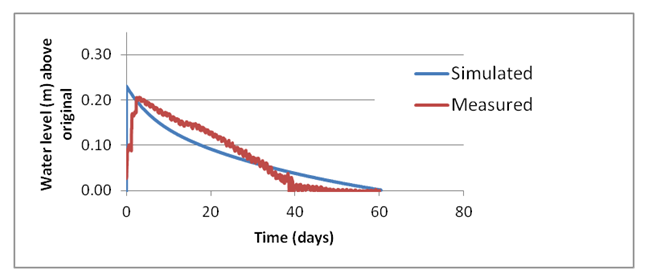
(Figure 32. Comparison between measured values (red color) and estimated values (blue color) for node 103. Tides were ignored in the simulation. The vertical axis represents deviations from the original level, which was due to an event that caused the anomaly in water level observations.)
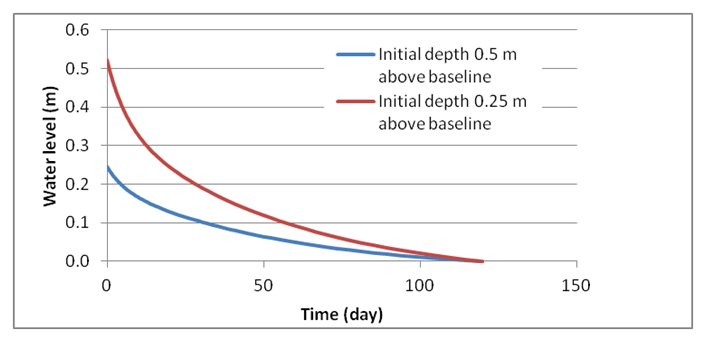
(Figure 33. Time decline in water level following its sudden rise above the baseline level.)
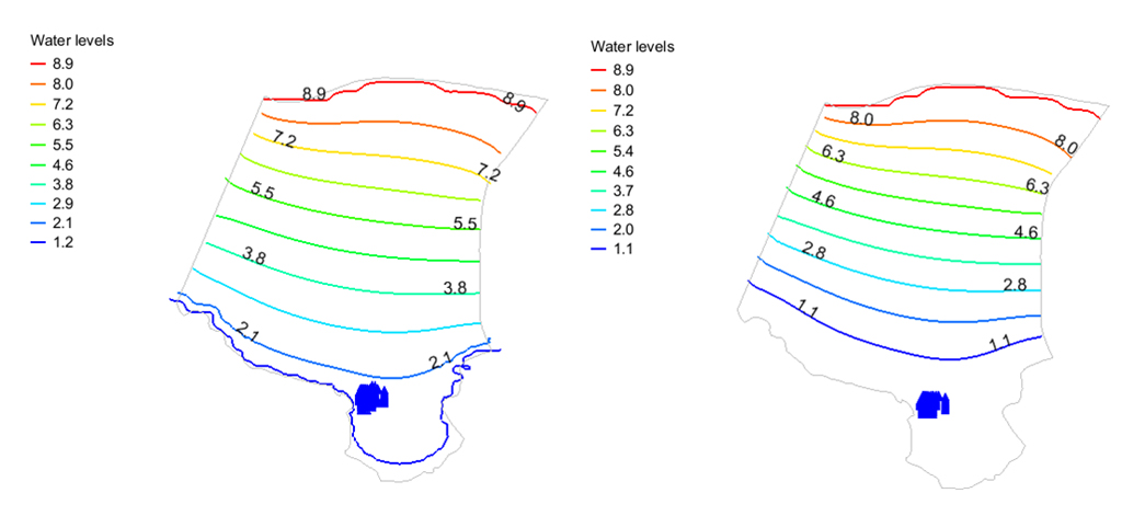
(Figure 34. Water levels under sea level rise (a) one meter, (b) 0.6 m. The blue area represents a flooded Pond under such scenarios. Overtopping is assumed not to occur (waves and erosion will likely exacerbate impacts). The colored lines are groundwater levels above msl.)
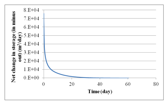
(Figure 35. Net change in the Pond storage due to inflows and outflows.)
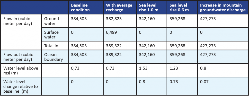
(Table 1. Steady state water budget for various scenarios. The flow in and out are referring to values entering and leaving the Pond, respectively. The water levels are referenced to the sea mean water level as well as to the baseline value.)


