APPENDIX 2. A Note About Modeling
Why Do We Need Models?
- Models are useful in understanding of water flow and chemical transport processes and for improving on theories.
- They are useful for the design field data collection schemes, emphasizing needed critical information
- They are used in a prediction mode to run numerical experiments (scenarios). They are more convenient and cheaper than real experiments. For example, I can add as many wells with a button click and analyze the consequences. Also models can be used to study future conditions before they occur.
Conceptual Model: A representation of a physical groundwater system, in this case the Pond and surrounding area. The conceptual model reflects our understanding of the system and can change based on available information and the objective of the study. The conceptual model can also change from one modeler to another. It includes various controlling processes, e.g., water flow and storage and chemical fate and transport.
Mathematical Model: Equations describing the controlling processes. For example, the equation describing water flux between two points is estimated based on the difference in water levels at the two points. Realistic equations are complex and change based on conceptualization as described above.
Numerical Models: Software used to solve the controlling equations based on the defined conceptual model. It is used first to calibrate the model and then to run numerical experiments (scenarios), such as what would be the response of the water level in the Pond to sea level rise.
The Modeling Process
- Identify specific modeling objectives, e.g., solve for water levels, salinity, contamination level, etc.
- Identify input variables and model needs
- Modeled area and conditions at the boundaries, such as ocean level or mountain discharge into the area
- Area divided in small cells where the solution would be estimated at the center of each cell.
- Aquifer data, such as permeability or hydraulic conductivity, which reflects the ease (or difficulty) of water movements, (called parameters). Some of these can be available (directly measured or inferred from available information). However, some might not be available or need adjustments through calibration (see below).
- Data for model calibration (see below), such as sensor water level data and salinities.3.Run the model to solve for variables under objectives
Model Calibration (Parameter estimation mode): Intended to gain confidence in the model. It is done by using available information (such as sensor readings) to estimate or improve on parameter estimates. The model is run many times to identify the parameter values that give the best match between measured and estimated data.
Model Use (Prediction Mode): Apply the model to address the modeling objectives (understanding, data collection, and scenario assessment).
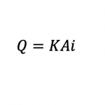
Hydraulic Conductivity versus Permeability: Flow is estimated by utilizing Darcy’s law (e.g., Fetter, 2018)[30], which is defined by:

In which Q is groundwater discharge through an area A under a slope of water table i. K is called hydraulic conductivity and has units of length per unit time (such as meter per day.) It reflects the ability of the aquifer to transmit water.
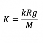
Conductivity is related to permeability k by:

In which R and M are the density and viscosity of water (or any liquid or gas) and g is acceleration of gravity. K is thus a function of the aquifer material and the type of liquid, while k (units of length, e.g., meter) is only a function of the aquifer material. As an example, k can be the same for a coastal aquifer, while K can change based on salinity, which affects water density.


